A digital elevation model of the Duplin River intertidal area
Final report submitted to the GCE-LTER Program
University of Georgia, Athens, GA
J. Blanton1
Skidaway Institute of Oceanography
Savannah, GA 31411
F. Andrade2
University of Lisbon, Faculty of Sciences
Marine Laboratory of Guia
Estrada do Guincho, 2750 Cascais PORTUGAL
M. Adelaide Ferreira3
IMAR-Marine Laboratory of Guia
Estrada do Guincho, 2750 Cascais PORTUGAL
I. Amft4
Skidaway Institute of Oceanography
Savannah, GA 31411
August 31, 2007
1e-mail: jack.blanton@skio.usg.edu
2email: f.andrade@ mail.telepac.pt
3e-mail: adelaiclferreira@mail.telepac.pt
4e-mail: julie.amft@skio.usg.edu
Introduction
Saltmarshes are intertidal areas which exhibit complex topographies of sloping flats cut by intricate networks of creeks. These areas are shaped primarily by hydrodynamics but also by biological and ecological factors (Mason et al., 2005). Topography, in turn, conditions and defines the vertical zonation of the saltmarsh and mudflat communities, by determining their immersion/emersion rhythms. Because saltmarshes were long considered wastelands (e.g., Chapman and Roberts (2004)), and because they were often inaccessible and difficult to survey using standard topographic techniques, little to no attention was given to the accurate cartography of those areas outside the main channels. To further complicate matters, these systems are very dynamic, usually rendering the available cartography obsolete, usually within a few years.
Detailed knowledge of the topography is necessary for accurate modelling of processes taking place on saltmarshes, Models to compute material exchange and biogeochemical phenomena require detailed information about the topography of the area and the amount of water stored in intertidal areas and released into the tidal channels and estuaries. Furthermore, vertical relief is also paramount in explaining the distribution and variability of the saltmarsh communities, namely halophytic vegetation.
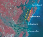
The GCE-LTER program is studying biogeochemical processes that change constituent concentrations in water as it flows over the marsh during flood tide and returns the modified water during ebb. The Duplin River is one of the focus areas for these studies (Fig. 1).
A high-resolution digital elevation model (DIEM) of the Duplin river, with a 1 m2 resolution, was constructed through the classification and analysis of a series aerial photographs sets taken during a flood tide. The rationale behind this method is:
- The flooded area can be objectively recognized
- The water surface is horizontal throughout the system and can therefore be used as a reference height (Lohani and Mason, 1999). This report describes the development and results of this DIEM
An aerial survey was conducted on 15 April 2004 to obtain data from which the topography of the Duplin River intertidal area could be derived. The survey consisted of a series of 7 passes over the Duplin River at 1-hr intervals, covering low water (LW) to high water (HW). For each pass, a total of eight images were obtained on infra-red (IR) film. The aircraft mission for the Duplin was conducted by Spectrum North Carolina, Inc. The images were scanned at 600 dpi to ensure a pixel resolution better than 1 m2, After being rectified to NADS3, TM-Zone 17, each RGB 24-bytes/pixel image (corresponding to three 8-bytes/pixel bands: blue (green on the film), green (red on the film) and the red (near-infrared on the film)), was processed to yield the water surface area as a function of time. Sub-surface pressure gages deployed along the tidal creek were used to determine the vertical reference level for the corresponding flooded area. The analyses of these images, reported here, yield a high-resolution digital elevation model (DIEM) of the intertidal area from which curves relating flooded area to water level can be constructed for the entire system of tidal creeks. The derivation of topography from images like these was successfully applied to a tidal creek in South Carolina (Blanton et al., 2006) with partial funding from NOAA’s Coastal Ocean Program.
Figure 1: Aerial image of the GCE-LTER domain. The yellow box defines the region covered by the aerial images.
Definition of intertidal drainage areas
The rectified LW image mosaic from the first aerial pass provided the base map used to define tidal creeks with LW widths of at least 5 m and determine their intertidal drainage areas. We used Wade Sheldon’s GCE Mapping Toolbox to
- Import the base image in UTM_NAD83 coordinates
- Digitize the basins
A careful examination of drainage zones around each creek provided the basis for drawing the divides separating the drainage area (polygon) of one creek from that of another. The implied assumption for each polygon is that no water causes the drainage boundaries. While some cross-boundary transport may occur at extreme high tides, the volumes involved are quite small compared to the volume of water in the intertidal areas that drains the surrounding creeks.
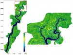
We defined 17 drainage areas using this procedure (Fig. 2), 12 of which have tributary tidal creeks (polygons 1-12) and corresponding catchment basins. The four without a creek (polygons 14, 15, 16 and 17) are assumed to transport mass into and out of their are as irregularly along the line separating them from the Duplin River, Polygon 13 is the main Duplin River at Low Water (LW) which ends 10 km upriver where the channel splits.
Figure 2: The definition of tidal tributaries and intertidal drainage areas for the Duplin River. The green polygons denote drainage areas having no creeks wider than 5 m. Easting and Northing axis values are given in meters.
Method to determine the DEM
Of the eight photo taken for each overflight, we selected the 5 that cover the Duplin drainage are a (photos 2 through 6) and the best-contrasted area in each photo. Each selected image was rectified to NAD83-TM17 datum with a 1-m by 1-m final resolution. The rectification process used a 2nd degree polynomial adjustment. This procedure allowed an exact superimposition of the selected images throughout the Duplin River domain and produced 7 mosaics of five photo access the 6-hr time interval, ordered from T7 (HW) to T1 (LW).
On each photo of the MW mosaic, an initial unsupervised classification of the ROB bands was conducted using KMEANS with a random seed for 75 classes. KMEANS is a clustering technique that partitions an image into K exclusive dusters. We always initialized KMEANS with K centroids (means) randomly distributed over the image (where K is defined by the analyst). Each pixel in the image is then assigned to the cluster whose centroid is nearest. Through an iterative process, cluster centroids are updated, and the process is repeated until the K centroids are fixed (Eastman, 2006). The analyst then determines which of the resulting clusters correspond to water and which do not.
All classes corresponding to flooded areas were reclassified to “1”. All remaining areas were reclassified to “0”, producing a “mask” for areas not flooded with water. Superimposing this mask to the corresponding T6 (HW-1h) photo retains only the flooded channels. This is the area that was then classified using KMeans with a random seed for 50 classes. The area classified in this step is much smaller and less heterogeneous (e.g., terrestrial areas have been totally excluded in the first step). A new mask was produced, now corresponding to the T6 flooded area, and the process of classifying flooded and non-flooded areas, of producing as mask and superimposing it to the previous image (in time) was repeated for times T6 through T1 (LW). This ensures an exact superimposition of successive flooded areas, from HW to LW.
The concatenation of all water classifications for each time (i.e., the LW to HW flooded area mosaics) enabled the quantification of flooded area for each time inside the overall Duplin drainage basin and inside each sub-basin (polygons 1-17). By assigning a vertical level to each flooded area, using measured tide heights at the corresponding over-flight times (Fig. 3), hypsometric curves (water area as a function of water elevation) and volume curves (stored volume as a function of water elevation) for the individual sub-basins and for the whole domain were constructed (file name = Hypso_subbasins.xls). We were then able to extract the outline for each individual water level/time (layer) to produce a three-dimensional file of X, Y (horizontal points on the NAD83-TM17 grid) and Z (m above MLW) for every point (1.7 x 10⁶) in these outlines. This file (Layer_L1mItsXYZdat) was used to construct a digital elevation model (DEM) for the intertidal domain of the Duplin River (file name = DEM_Duplin_all.tif)) using a universal Krigging interpolation algorithm (Fig. 4). See file SKIO_24_8_07.pdf for more details on the methodogy.
Discussion of hypsometric curves and tidal prisms
The file Hypso_subbasins.xls contains the hypsometric curves for each polygon and for the entire Duplin River intertidal area. A comparison of four polygon curves indicates some general trends in intertidal morphology (Fig. 5). The LW starting point (-0.10 m) of these curves shows the LW (Ti) area in each polygon. The water level of 2.19 m is the highest level observed for the neap tide of 15 April 2004 (an unusually large neap tide). The maximum water level (2.32 m) is the mean higher high water (MHHW) value given in the NOAA Tide Tables for “Old Tower” station. Water at this level is assumed to completely cover the intertidal area. Therefore, the maximum areas in Figure 5 are simply the size of the polygons.
Poly 16 (no creek > 5 m wide) has practically no water inside until water level passes 2 m. Further water rise indicates a spread in area to the maximum size of the polygon. This polygon is typical of the other “no-creek” polygons (14,15,17) except that water area in “17” begins to grow when water level rises above 1.2 m. Curves for Polygons “5” and “6” are typical of those intertidal areas having drainage creeks wider than 5 m. While the LW areas differ over a large range, the rate of water level growth is similar and begins rather early in the tidal stage. In general, the rate of growth is smaller in the intertidal areas south of Hunt Camp. That all areas begin to grow rapidly after reaching the 2-m level indicates that the water leaves confining channels late in the flood phase.
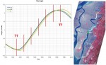
Figure 3: Water level curves for 15 April 2004 at along the axis of the Duplin River The red vertical lines (T1 through T7) show the times of each aerial pass. The locations of the three curves are shown in the image on the right. Water level at a given time varies within 0.1 m over a distance of ~7 km, so water surface is assumed to be horizontal over the 2-min duration of a single pass of the airplane. Data courtesy of Dr. Daniela Di Iorio and the LTER monitoring network.
The total volume between LW and HW represents the tidal prism. Plots of volume versus water level give representations of growth and size of prisms throughout the study domain (Fig. 6). Eleven of 16 prisms show relatively slow growth rates and small initial volumes. The largest tidal prisms are found for Polygon 1 (Barn Creek) and Polygon 5 (Marsh along the east fork north of Hunt Camp.
Careful study of the individual hypsometric curves as well as those describing the growth in water volume (also on file Hypso.subbasins.xls) is likely to reveal morphological details through out the Duplin River intertidal area that would be relevant to the distribution of plants and animals as well as residence time of water. Numerical models of water circulation in the river may simulate tidal currents more accurately by incorporating the DEM (file Layer_Limits_XYZ.dat) into their mesh.
Figure 4: Digital elevation model of the intertidal area surrounding the Duplin River. The right-hand figure is a detailed view of the area north of Hunt Camp.
Conclusions
The method applied here demonstrates that morphology and elevation of intertidal areas of the size surrounding the Duplin River can be defined to resolutions as high as 1 m2. Even without direct ground-truthing, results are much more informative than previously available data. The hypsometric curves (Fig. 5) have a consistent pattern of growth in water level versus time based on following the evolution of water area during a flood tide.
Uncertainties lie mostly with the capacity to detect thin layers of water on the most dense marshes. One of the more serious limitations is that ground truthing is virtually impossible in these environments. Marsh surfaces are treacherous to navigate on foot and to physically mount 10-20 targets in the areas north of Hunt Camp would be arduous and costly.
We submit that a similar definition of water area and volume as a function of water level during the ebb phase of the tidal cycle would yield a new level of information. The ebb/flood hypsometric curves and corresponding tidal prisms are likely to vary throughout the Duplin intertidal area, a variation that is likely to shed light on substrate differences and density of peripheral tidal channels throughout the area.
Figure 5: A comparison of hypsometric curves for four polygons with the total drainage area. The final line-segment in each plot connects water depths and areas from 2.19 to 2.30 meters. The area at 2.19 m references the largest water area calculated for the final overflight (T7). The area at 2.30 m (the water level of the NOAA-published mean spring HHW) references the total polygon area. Areas for the total Duplin tidal water shed have been divided by ten to scale that curve with the polygons.
Figure 6: A comparison of tidal prisms for all polygons (Fig. 2). Northern prisms are on the left; southern prisms are on the right. Each curve starts 1 hr after LW (T2), beginning with the volume stored in the first 1-hr interval. The final line-segment in each plot connects water depths and areas from 2.19 to 2.32 meters. The area at 2.19 m references the largest volume calculated for the final image set (17). The volume at 2.32 m references the total polygon area. Volumes for the total Duplin tidal water shed have been divided by ten to scale that curve with those of the polygons.
Acknowledgments
Our thanks go to Daniela Di Iorio, Paul McKay and Ken Helm who provided the sub-surface pressure data along the axis of the Duplin that enabled us to relate image time to water level. We thank Mike Robinson at Skidaway Institute of Oceanography for doing preliminary calculations of water areas used in the 2007 Progress Report, and Clark Alexander for presenting the preliminary results at the GCE-LTER 2007 annual meeting. Our thanks also go to Steven Pennings and Tim Hollibaugh for their support to develop the DEM for the Duplin River.
We acknowledge funding from the National Science Foundation (OCE 99-821 33) which funded the aerial mission to gather the infrared images as well as the analyses reported here. We also acknowledge funding the Luso-America Foundation (FLAD), which contributed to the support of F. Andrade and M.A, Ferreira.
References
Blanton, J., Andrade, F., and Ferreira, M, A. (2006). The relationship of hydrodynamics and morphology in tidal-creek and salt-marsh systems in South Carolina and Georgia. In Kleppel, G., DeVoe, M., and M.V. Rawson, J., editors, Implications of Changing Land Use Patterns to Coastal Ecosystems. Springer-Verlag, New York, USA.
Chapman, M. and Roberts, D. (2004). Use of seagrass wrack in restoring disturbed Australian saltmarshes. Ecological Management and Restoration, 5(3):183—190.
Eastman, J. (2006). JDRJSI Andes: Guide to GIS and image Processing. Clark Labs, Clark University.
Lohani, B. and Mason, D. (1999). Construction of a digital elevation model of the holderness coast using the waterline method and airborne thematic mapper data, Int. J. Remote Sensing, 20(3):593—607.
Mason, D., Marani, M., Belluco, E., Feola, A., Ferrari, S., Katzenbeisser, R., Lohani, B., Menenti, M., Paterson, D., Scott, T., Vardy, S., Wang, C., and Wang, H.-J. (2005). Lidar mapping of tidal marshes for ecogeomorphological modelling in the tide project. In Eighth International Conference on Remote Sensing for Marine and Coastal Environments, Halifax, Nova Scotia, 17-19 May.
http://gce-lter.marsci.uga.edu/lter/research/tools/it_development.htm
This PDF version is the full, original version of this report and contains content not previously published in the the print version of the Spring 2005 Network Newsletter.
 Enlarge this image