Comparative Analysis of Spatial Heterogeneity of LTER Landscapes

A Progress Report after Year One

This intersite study of spatial heterogeneity and scaling at landscape levels is founded on the assertion that the temporal behavior of ecological systems is greatly influenced by their spatial structure. We think that it is time in the LTER Program to develop our landscape perspective of spatial heterogeneity to generate hypotheses as to how this property will interact with the temporal behavior of our set of disparate ecosystems. Such studies may help guide ecologists in attempts to understand and predict the behavior of ecological systems at regional and global levels and help generate new concepts and hypotheses at a more general level than can be achieved from smaller scale studies at single LTER sites.

Comparisons of spatial heterogeneity are greatly biased by the tools of measurement. Ecologists working in lake, ocean, and various land systems use instruments that observe at different resolution or grain. Although this scale dependency poses problems for comparisons of diverse systems, it also presents opportunities for advancing ecological understanding using the new tools available. Use of remotely sensed multi-spectral spatial data from Landsat now provides an opportunity to observe divergent ecological systems at the same grain and at nested spatial scales. This is an early and necessary step in comparative landscape ecology at a network level. Remote sensing provides the only tool available for making across-site comparisons at the same nested sets of spatial scales. The satellite data set is one of only two or three data sets standardized across the entire LTER Network.

With an NSF Mid-Career Fellowship (see Network News issue 12), John Magnuson spent 1992 at the LTER Network Office initiating inquiry on the following questions in collaboration with John Van de Castle and Mark MacKenzie:

• How do our LTER sites order along a gradient of low to high spatial heterogeneity?
• How does the ordering of the LTER sites From low to high spatial heterogeneity change with spatial scale of observation, both grain and extent? 
• What is the explanation for the order of each site along the gradient of low to high spatial heterogeneity? 
• How well do the LTER sites represent the spatial heterogeneity of the regions in which they occur?

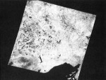
The parameters we are using to compare spatial heterogeneity are the coefficients of variation of vegetation indices measured using radiance values of the red and near-infrared bands (TM bands 3 and 4). These values have been calculated based on 28.5-m pixels for entire Landsat scenes 180 km by 130 km in extent. The scenes were also masked to remove pixels of cloud, shade, water, snow, and ice in various combinations. The order of the sites from high to low spatial heterogeneity was similar for both the vegetation index and the normalized vegetation index. Removing cloud and shade noticeably reduced heterogeneity within some scenes. Removing water pixels greatly reduced the estimates of spatial heterogeneity at several sites, such as the Seattle area and North Temperate Lakes. Removal of ice and snow slightly reduced the estimate of spatial heterogeneity in scenes containing the Bonanza Creek LTER site in central Alaska and the Seattle scene that included Mount Rainier and the North Cascades.

The most intriguing preliminary result to date from our 12-site analysis of the 1991 Landsat images is that the differences in spatial heterogeneity of the entire images containing LTER sites do not order from high to low spatial heterogeneity by any obvious intuitive differences among the regions. Spatial heterogeneity of the land portions of the scenes does not order by latitude, precipitation, geological relief, or biome type. For example, when only the land portions of the scenes are considered, an agricultural scene (KBS) is the most variable and a desert scene (JRN) is the second most variable, while the least variable scene is a dry grassland (SEV) and the second least variable scene is a mixed Great Lakes forest (NTL).

Preliminary analysis of two scenes at nested spatial scales of resolution from 28.5-m to 10-km pixels in one-pixel steps confirms that the coefficient-of-variation measure of spatial heterogeneity declines rapidly with increasing pixel size. The expectation is that the scenes will order differently at different scales of resolution. For example, much of the heterogeneity at the Kellogg Biological Station agricultural site is at the scale of whole agricultural fields and, once the pixel size is aggregated to a size greater than individual fields, the heterogeneity should decline sharply for that site.

The long-term goals of this research are to:

• Describe and compare spatial heterogeneity of disparate landscapes

• Explain the similarities and differences among disparate landscapes

• Determine whether such similarities and differences in spatial heterogeneity influence ecological functioning and processes at regional levels irrespective of the landscape type

• Determine whether there is a role for such information in management, protection, and restoration at regional levels. Significant progress on the first two of these goals was made during 1992, although several calibration and programming problems remain in our analysis.

The second objective is of special interest because the differences in spatial heterogeneity of the scenes did not order with respect to biome type and related climate or geological relief. We hope to complete these analyses during the next year. The final two objectives are long-term goals of ecologists in general and will continue to challenge us all to better understand and interact with the world around us.

For more information:

John J. Magnuson, Center for Limnology, University of Wisconsin, 680 North Park Street, Madison, Wisconsin 53706 608-262-3014, jMagnuson@LTERnet.edu.